Software Setup
This year, the recommended way to work on assignments is through Google Colaboratory. However, if you already own GPU-backed hardware and would prefer to work locally, we provide you with instructions for setting up a virtual environment.
Working remotely on Google Colaboratory
Google Colaboratory is basically a combination of Jupyter notebook and Google Drive. It runs entirely in the cloud and comes preinstalled with many packages (e.g. PyTorch and Tensorflow) so everyone has access to the same dependencies. Even cooler is the fact that Colab benefits from free access to hardware accelerators like GPUs (K80, P100) and TPUs which will be particularly useful for assignments 2 and 3.
Requirements. To use Colab, you must have a Google account with an associated Google Drive. Assuming you have both, you can create a new Colab notebook by visiting Google Colaboratory. When you open the webpage, it will prompt you to create a new notebook. Click on the Google Drive tab and click New notebook. Then you will be able to use Colab.
You can also upload your notebooks to Google Drive. In order to open the notebooks in with Colab,
- Right click on the file name.
- Click on
Open with->Connect more apps. - Search Colaboratory in
Google Workspace Marketplace. - Install
Colaboratory.
One you successfully install Colab, you can right click on your notebooks and open them with the app.
Workflow. Every assignment provides you with a download link to a zip file containing Colab notebooks and Python starter code. You can upload the folder to Drive, open the notebooks in Colab and work on them, then save your progress back to Drive. We encourage you to watch the tutorial video below which covers the recommended workflow using assignment 1 as an example.
The video is made specific to Standford CS231n and can be adapted to our course
Best Practices. There are a few things you should be aware of when working with Colab. The first thing to note is that resources aren’t guaranteed (this is the price for being free). If you are idle for a certain amount of time or your total connection time exceeds the maximum allowed time (~12 hours), the Colab VM will disconnect. This means any unsaved progress will be lost. Thus, get into the habit of frequently saving your code whilst working on assignments. To read more about resource limitations in Colab, read their FAQ here.
Using a GPU. Using a GPU is as simple as switching the runtime in Colab. Specifically, click Runtime -> Change runtime type -> Hardware Accelerator -> T4 GPU and your Colab instance will automatically be backed by GPU compute.
If you’re interested in learning more about Colab, we encourage you to visit the resources below:
Working locally on your machine
If you do not want to use Google Colaboratory and wish to work locally, you should use a virtual environment. You can install one via Anaconda (recommended) or via Python’s native virtualenv module. Ensure you are using Python 3.10 as we are no longer supporting Python 2.
Anaconda virtual environment
We strongly recommend using the free Anaconda Python distribution, which provides an easy way for you to handle package dependencies. Please be sure to download the Python 3 version, which currently installs Python 3.10. The neat thing about Anaconda is that it ships with MKL optimizations by default, which means your numpy and scipy code benefit from significant speed-ups without having to change a single line of code.
Once you have Anaconda installed, it makes sense to create a virtual environment for the course. If you choose not to use a virtual environment (strongly not recommended!), it is up to you to make sure that all dependencies for the code are installed globally on your machine. To set up a virtual environment called compsci682, run the following in your terminal:
# this will create an anaconda environment
# called compsci682 in 'path/to/anaconda3/envs/'
conda create -n compsci682 python=3.10
To activate and enter the environment, run conda activate compsci682. To deactivate the environment, either run conda deactivate compsci682 or exit the terminal. Note that every time you want to work on the assignment, you should rerun conda activate compsci682.
# sanity check that the path to the python
# binary matches that of the anaconda env
# after you activate it
which python
# for example, on my machine, this prints
# $ '/Users/kevin/anaconda3/envs/sci/bin/python'
You may refer to this page for more detailed instructions on managing virtual environments with Anaconda.
Note: If you’ve chosen to go the Anaconda route, you can safely skip the next section and move straight to Installing Packages.
Manual install, virtual environment
If you’d like to (instead of Anaconda) go with a more manual and risky installation route you will likely want to create a virtual environment for the project. If you choose not to use a virtual environment, it is up to you to make sure that all dependencies for the code are installed globally on your machine. To set up a virtual environment, run the following:
For Linux / MacOS
cd cs682
conda create -n compsci682 python=3.10	# Create environment
conda activate compsci682				# Activate the environment
pip install -r requirements.txt		# Install dependencies
conda install jupyter			 # Install Jupyter
# Work on the assignment for a while ...
deactivate                       # Exit the virtual environment
For Windows
cd cs682
conda create -n compsci682 python=3.10	# Create environment
conda activate compsci682				# Activate the environment
pip install -r requirements.txt		# Install dependencies
# Work on the assignment for a while ...
deactivate                       # Exit the virtual environment
Installing packages
Once you’ve setup and activated your virtual environment (via conda or venv), you should install the libraries needed to run the assignments using pip. To do so, run:
# again, ensure your virtual env (either conda or venv)
# has been activated before running the commands below
cd assignment1  # cd to the assignment directory

# install assignment dependencies.
# since the virtual env is activated,
# this pip is associated with the
# python binary of the environment
pip install -r requirements.txt
Jupyter Setup
In this class, you may use Jupyter Notebook to work on the programming assignments locally. A Jupyter notebook lets you write and execute Python code in your web browser. Jupyter notebooks make it very easy to tinker with code and execute it in bits and pieces; for this reason Jupyter notebooks are widely used in scientific computing.
Installing and running Jupyter is easy. From the command line, the following will install Jupyter:
pip install jupyter
Or the following if you use conda/Anaconda:
conda install jupyter
Once you have Jupyter installed, start it with this command:
jupyter notebook
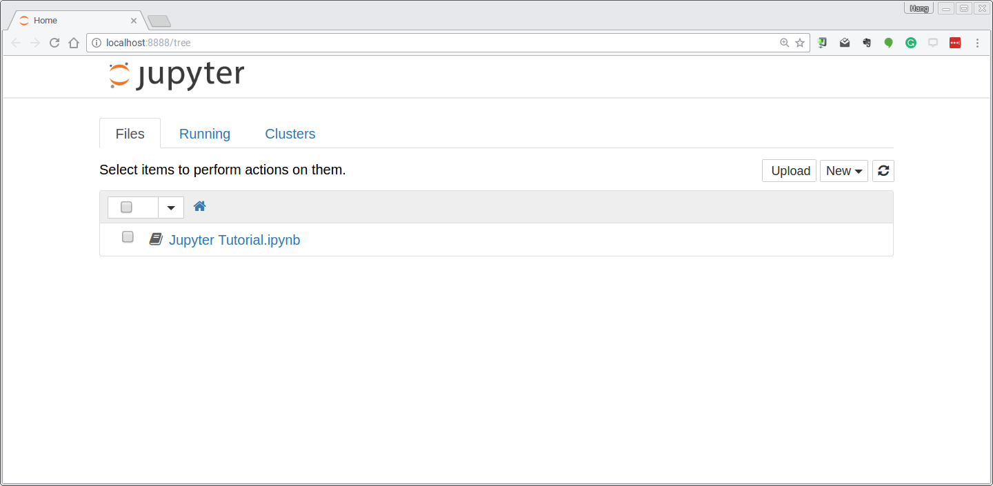
Once Jupyter is running, point your web browser at http://localhost:8888 to start using Jupyter notebooks. If everything worked correctly, you should see a screen like this, showing all available Jupyter notebooks in the current directory:
If you click through to a notebook file, you will see a screen like this:
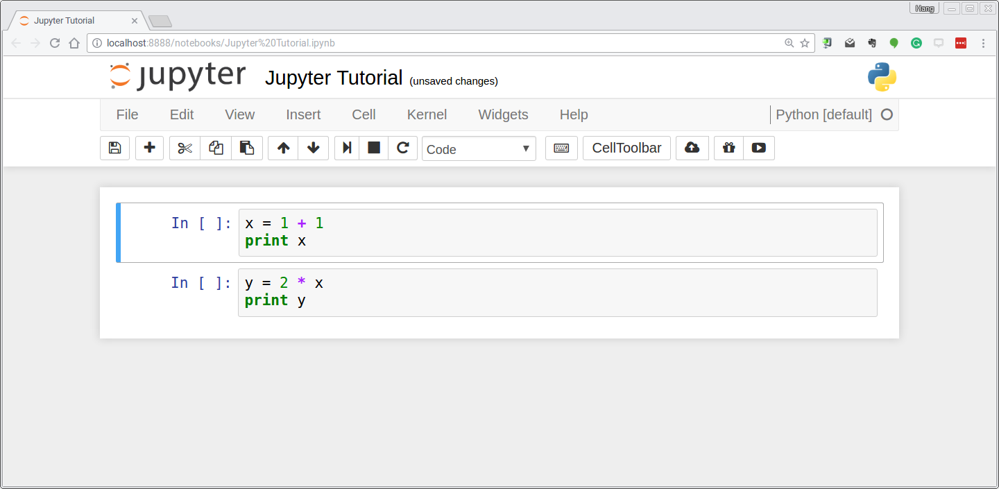
A Jupyter notebook is made up of a number of cells. Each cell can contain
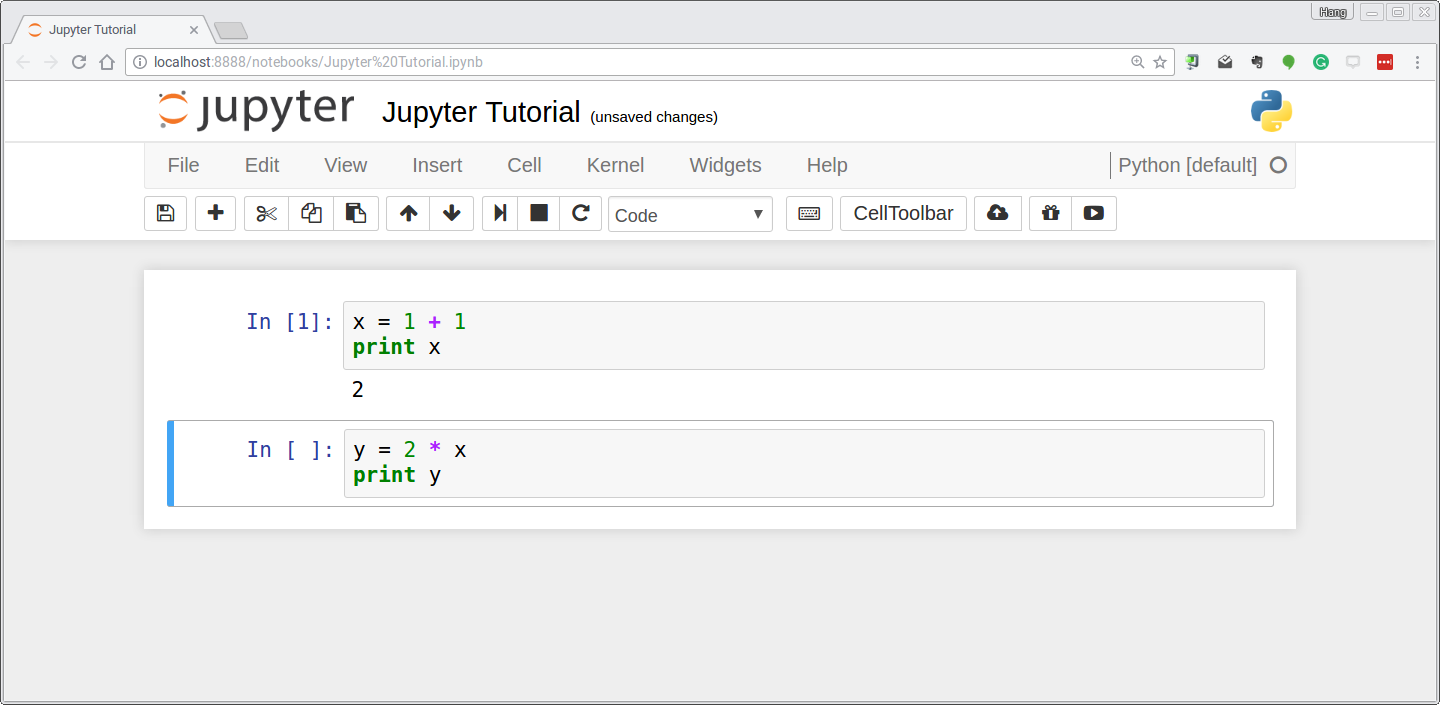
Python code. You can execute a cell by clicking on it and pressing Shift-Enter.
When you do so, the code in the cell will run, and the output of the cell
will be displayed beneath the cell. For example, after running the first cell
the notebook looks like this:
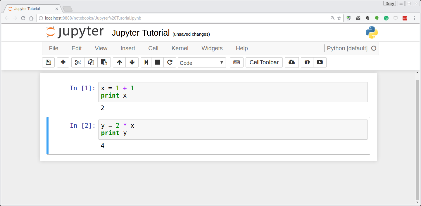
Global variables are shared between cells. Executing the second cell thus gives the following result:
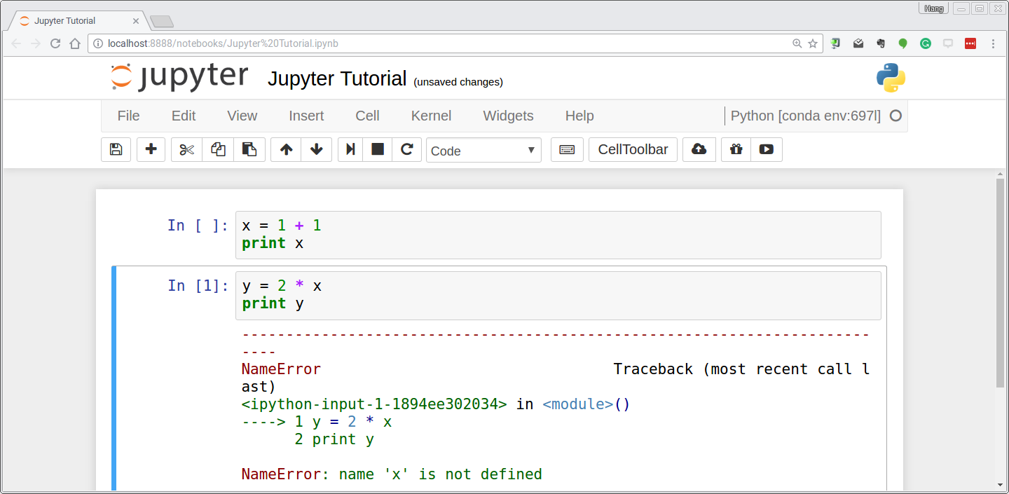
By convention, Jupyter notebooks are expected to be run from top to bottom. Failing to execute some cells or executing cells out of order can result in errors:
After you have modified a Jupyter notebook for one of the assignments by modifying or executing some of its cells, remember to save your changes!
This has only been a brief introduction to Jupyter Notebook, but it should be enough to get you up and running on the assignments for this course. Check out these notebooks if you want to learn more.